
Implementation and Empirical Analysis of Multi-Armed Bandit Problem
Published:
![]()
Welcome to my latest blog post! Today, I am excited to share my recent exploration into the fascinating world of reinforcement learning, specifically focusing on the multi-armed bandit problem and its various solutions. As a foundation for my implementation, I closely followed the insightful book, Reinforcement Learning: An Introduction (second edition) by Richard S. Sutton and Andrew G. Barto. In this post, I will walk you through my journey, discussing key concepts and algorithms presented in Chapter 2 of the book, while also providing you with code examples and explanations to help you grasp these intriguing topics. So, let’s dive into the world of multi-armed bandits and reinforcement learning together!
Multi-Armed Bandit Problem
The Multi-Armed Bandit problem is a classic reinforcement learning challenge that exemplifies the exploration-exploitation tradeoff dilemma. Imagine a gambler(an agent in terms of RL terminology) in front of a row of slot machines, also known as “one-armed bandits.” The gambler needs to decide which machines to play, how many times to play each machine, in which order to play them, and whether to continue with the current machine or try a different one. Each machine provides a random reward from a probability distribution specific to that machine, which is unknown to the gambler. The objective is to maximize the sum of rewards earned through a sequence of lever pulls.
The critical tradeoff the gambler faces at each trial is between “exploitation” of the machine that has the highest expected payoff and “exploration” to gather more information about the expected payoffs of the other machines. In practice, multi-armed bandits have been used to model problems such as managing research projects in a large organization or optimizing marketing strategies.
In the following sections, I will delve into the implementation of the Multi-Armed Bandit problem. This implementation will follow the order of problems and solutions presented in the book by Sutton and Barto. Throughout this process, I will make an effort to compare the performance of various algorithms with each other, allowing us to evaluate their effectiveness in addressing the exploration-exploitation tradeoff.
Let’s begin by importing the libraries and setting them up!
import numpy as np
import matplotlib
import matplotlib.pyplot as plt

# For each multiarmed bandit experiment we'll have two plots, displayed horizontally
matplotlib.rcParams['figure.figsize'] = [20, 5]
matplotlib.rcParams['axes.prop_cycle'] = matplotlib.cycler(color=['g', 'b', 'r', "y"])
Stationary Multi-Armed Bandit
The simplest setting for the multi-armed bandit problem is when the reward for choosing an arm remains constant over time. In this scenario, each arm has a fixed probability distribution for its rewards, and the gambler’s objective remains the same: to maximize the cumulative reward over a series of trials.
class StationaryMultiArmedBandit:
    """
    Represents a stationary multi-armed bandit problem.

    Attributes:
        k (int): Number of arms.
        runs (int): Number of independent runs.
        random_state (int, optional): Random seed for reproducibility.
    """
    def __init__(
            self,
            k,
            runs,
            random_state=None,
    ):
        self.k = k
        self.runs = runs
        self.random_state = random_state

        self.setup()

    def setup(self):
        """Set up the seed for reproducibility and reward distribution"""
        self.nprandom = np.random.RandomState(self.random_state)
        self.q_star = self.nprandom.normal(
            loc=0.0,
            scale=1.0,
            size=(self.runs, self.k),
        )

    def get_reward(self, action):
        """Given the action, return the reward"""
        reward = self.nprandom.normal(
            loc=self.q_star[np.arange(self.runs), action],
            scale=1.0,
        )
        return reward

    def get_correct_action(self):
        """
        Get the correct action for each run.
        Correct action for each run is the one with highest mean reward
        """
        return self.q_star.argmax(axis=1)

    def plot_reward_distribution(self, run=0):
        """Plot the reward distribution for the given run."""
        samples = self.nprandom.normal(
            loc=self.q_star[run],
            scale=1.0,
            size=(10_000, self.k),
        )
        plt.violinplot(samples, showmeans=True)
        plt.xlabel('Action')
        plt.ylabel('Reward Distribution')
        plt.show()
For all experiments, we’ll aggregate the performance across 2000 independent 10-armed bandit runs. Let’s create variables to store these numbers.
runs = 2000
k = 10
Now let’s create an instance of Stationary Multi-Armed Bandit problem, and see its reward distribution. The agent will be unknown to this reward distribution. The ideal agent should be able to learn the correct action that gives the highest reward.
st_bandit = StationaryMultiArmedBandit(k=k, runs=runs)
st_bandit.plot_reward_distribution(run=0)
print(f"Correct action for run 0: {st_bandit.get_correct_action()[0] + 1}")
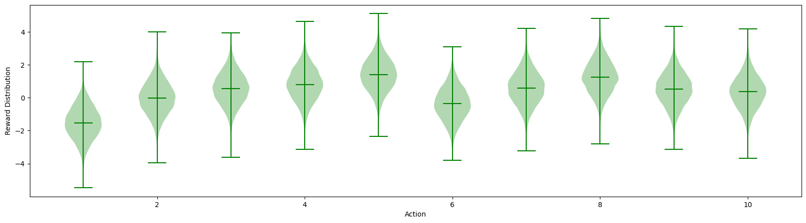
Correct action for run 0: 5
Agent
An agent in reinforcement learning is an entity that learns the actions that yield the highest reward in the long run. The agent has two primary roles:
- acting on the environment based on the current estimate of action values and
- updating the action values estimate based on the rewards it receives.
One of the challenges faced by the agent is the exploration-exploitation dilemma. In this dilemma, the agent must decide whether to explore new actions to gain more knowledge about the environment or exploit its current knowledge to maximize immediate rewards. Striking a balance between exploration and exploitation is critical for the agent’s success in the long run, as excessive exploration may lead to suboptimal rewards, while excessive exploitation may prevent the agent from discovering better actions. Various types of agents can be developed based on how they handle this exploration-exploitation trade-off, and in our implementation, we will compare different methods to understand their effectiveness in addressing this challenge.
Epsilon Greedy Sample Average Agent
The epsilon-greedy sample average method addresses the exploration-exploitation dilemma by choosing between exploration and exploitation randomly. With a probability of epsilon, the agent selects a random action for exploration, while with a probability of 1-epsilon, the agent exploits the current best action based on its estimated action values.
In comparison to the pure greedy algorithm, which always selects the action with the highest estimated value, the epsilon-greedy algorithm introduces a level of exploration, allowing the agent to discover potentially better actions and improve its long-term performance.
The sample average estimate is a technique used to update the estimated action values. For each action, the agent maintains a running average of the rewards it has received when selecting that action. When a new reward is received, the agent updates its estimate by incorporating the new reward into the running average. This way, the agent continuously refines its estimates based on its experience, which in turn helps it make better decisions in the exploration-exploitation trade-off.
class EpsilonGreedySampleAverageAgent:
    """
    An epsilon-greedy agent using sample-average method for action value estimation.

    Attributes
    ----------
    k : int
        Number of actions.
    runs : int
        Number of independent runs.
    epsilon : float, optional
        Probability of choosing a random action (exploration), default is 0.1.
    random_state : int, optional
        The random number generator seed to be used, default is None.
    """
    def __init__(
            self,
            k,
            runs,
            epsilon=0.1,
            random_state=None,
    ):
        self.k = k
        self.runs = runs
        self.epsilon = epsilon
        self.random_state = random_state

        self.setup()

    def setup(self):
        """Initialize the Q and N arrays for action value estimation and action counts."""
        self.nprandom = np.random.RandomState(self.random_state)
        self.Q = np.zeros((self.runs, self.k))
        self.N = np.zeros((self.runs, self.k))

    def get_action(self):
        """Choose an action based on epsilon-greedy policy."""
        greedy_action = np.argmax(
            self.nprandom.random(self.Q.shape) * (self.Q==self.Q.max(axis=1, keepdims=True)), # breaking ties randomly
            axis=1
        )
        random_action = self.nprandom.randint(0, self.k, size=(self.runs, ))

        action = np.where(
            self.nprandom.random((self.runs, )) < self.epsilon,
            random_action,
            greedy_action,
        )
        return action

    def get_step_size(self, action):
        """Calculate the step size for updating action value estimates.
        For sample average method we return 1/number of times the action is choosen until current step"""
        return 1/self.N[np.arange(self.runs), action]

    def update(self, action, reward):
        """Update the action value estimates based on the chosen action and received reward."""
        self.N[np.arange(self.runs), action] += 1
        step_size = self.get_step_size(action)
        self.Q[np.arange(self.runs), action] += (reward - self.Q[np.arange(self.runs), action])*step_size
Now, we’ll create a testbed which will a run episode of parley between agent and k-arm bandit environment for the provided number of steps. We’ll also include a function that plots the average reward agent is receiving and percentage optimal action the agent is taking in each steps.
class MultiArmedBanditTestBed:
    """A test bed for running experiments with multi-armed bandits and agents.

    Attributes:
        bandit (object): A multi-armed bandit object.
        agent (object): An agent object.
        steps (int): The number of steps for the experiment.
    """
    def __init__(
            self,
            bandit,
            agent,
            steps,
    ):
        self.bandit = bandit
        self.agent = agent
        self.steps = steps

    def run_experiment(self):
        """Runs the experiment for the given number of steps and returns the average rewards and optimal actions.

        Returns:
            tuple: A tuple containing two lists: average rewards and average optimal actions for each step.
        """
        avg_reward = []
        avg_optimal_action = []

        for _ in range(self.steps):
            action = self.agent.get_action()
            reward = self.bandit.get_reward(action)
            self.agent.update(action, reward)

            correct = action == self.bandit.get_correct_action()

            avg_reward.append(reward.mean())
            avg_optimal_action.append(correct.mean())

        return avg_reward, avg_optimal_action

    @classmethod
    def run_and_plot_experiments(cls, steps, exp_bandit_agent_dict):
        """Runs multiple experiments and plots the results.

        Args:
            steps (int): The number of steps for the experiments.
            exp_bandit_agent_dict (dict): A dictionary with labels as keys and (bandit, agent) tuples as values.
        """
        fig, (ax_reward, ax_optimal_action) = plt.subplots(nrows=1, ncols=2)

        for label, (bandit, agent) in exp_bandit_agent_dict.items():
            test_bed = cls(bandit, agent, steps)
            avg_reward, avg_optimal_action = test_bed.run_experiment()
            ax_reward.plot(avg_reward, label=label)
            ax_optimal_action.plot(avg_optimal_action, label=label)

        ax_reward.set_ylabel("Average reward")
        ax_reward.set_xlabel("Steps")

        ax_optimal_action.set_ylabel("% Optimal Action")
        ax_optimal_action.set_xlabel("Steps")

        ax_reward.legend()
        ax_optimal_action.legend()

        plt.show()
Experiment 1: Greedy Vs \(ϵ\)-Greedy
Let’s run three agents: greedy, \(\epsilon=0.1\)-greedy, and \(\epsilon=0.01\)-greedy agent on the stationary 10-arm bandit environment.
MultiArmedBanditTestBed.run_and_plot_experiments(
    steps=10_000,
    exp_bandit_agent_dict={
        "greedy": (
            StationaryMultiArmedBandit(k=k, runs=runs),
            EpsilonGreedySampleAverageAgent(k=k, runs=runs, epsilon=0)
        ),
        "epsilon=0.1": (
            StationaryMultiArmedBandit(k=k, runs=runs),
            EpsilonGreedySampleAverageAgent(k=k, runs=runs, epsilon=0.1)
        ),
        "epsilon=0.01": (
            StationaryMultiArmedBandit(k=k, runs=runs),
            EpsilonGreedySampleAverageAgent(k=k, runs=runs, epsilon=0.01)
        ),
    },
)
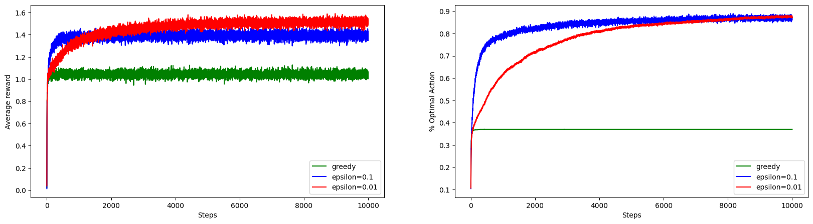
In the plots above, we can clearly see that epsilon greedy agent outperforms the pure greedy agent because greedy agent did no exploration and got stuck on the suboptimal action. On comparing the two epsilon greedy agent, we can see that agent with higher epsilon explored more and got better performance at initial stage. But, the agent with low epsilon value outperforms the agent with high epsilon agent in the long run. This clearly show the challenges of finding the balance between exploration and exploitation.
Non-Stationary Multi-Armed Bandit Problem
Let’s shift the multi-armed bandit problem a bot towards a realistic full reinforcement learning paradigm. The bandit implemented earlier was stationary as its reward distribution never changed during its lifetime. Let’s implement a bandit where the reward distribution changes with steps the agent takes.
class NonStationaryMultiArmedBandit(StationaryMultiArmedBandit):
    def setup(self):
        """For stationary bandit, we start with same average reward for all actions. Let's say zero."""
        self.nprandom = np.random.RandomState(self.random_state)
        self.q_star = np.zeros((self.runs, self.k))

    def get_reward(self, action):
        """Before getting reward for the action taken in the current step,
        we shift the reward distribution with drift sampe from normal distribution with mean 0 and std 0.01"""
        self.q_star += self.nprandom.normal(loc=0.0, scale=0.01, size=(runs, k))
        return super(NonStationaryMultiArmedBandit, self).get_reward(action)
Experiment 2: Sample Average Action Value Estimation Method on Stationary and Non-Stationary Problem
MultiArmedBanditTestBed.run_and_plot_experiments(
    steps=10_000,
    exp_bandit_agent_dict={
        "stationary": (
            StationaryMultiArmedBandit(k=k, runs=runs),
            EpsilonGreedySampleAverageAgent(k=k, runs=runs, epsilon=0.01)
        ),
        "nonstationary": (
            NonStationaryMultiArmedBandit(k=k, runs=runs),
            EpsilonGreedySampleAverageAgent(k=k, runs=runs, epsilon=0.01)
        ),
    },
)
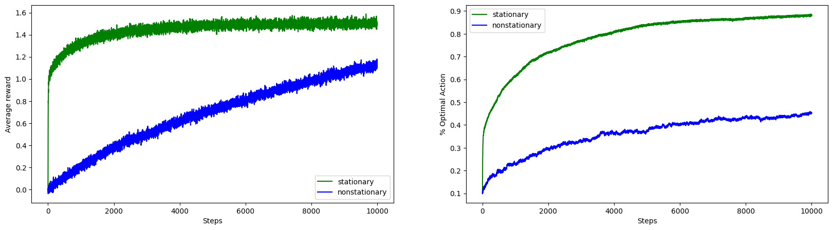
It is clearly seen that for non stationary bandit problem sample average method falls significantly behind.
Epsilon Greedy with Constant Step Size
The sample average method gives equal weightage to reward obtain irrespective of the steps in which they were obtained. However, in case of nonstationary setting it makes sense to give more weight to recent rewards than to long-past rewards. One of the most popular ways of doing this is to use a constant step-size parameter.
class EpsilonGreedyAgent(EpsilonGreedySampleAverageAgent):
    """Epsilon greedy agent with constant step size."""
    def __init__(self, k, runs, alpha=0.1, epsilon=0.1, random_state=None):
        super(EpsilonGreedyAgent, self).__init__(k, runs, epsilon, random_state)
        self.alpha = alpha

    def get_step_size(self, action):
        """Instead of returning number of times the action is choosen,
        it returns the constant step size `alpha` provided to agent during its instantiation."""
        return self.alpha
Experiment 3: Epsilon Greedy with Constant Step-Size in Non-Stationary Environment
Let’s run experiment with combinations of stationary/non-stationary bandit and sampleaverage/constant step size action value estimation methods.
MultiArmedBanditTestBed.run_and_plot_experiments(
    steps=10_000,
    exp_bandit_agent_dict={
        "stationarysampleaverage": (
            StationaryMultiArmedBandit(k=k, runs=runs),
            EpsilonGreedySampleAverageAgent(k=k, runs=runs, epsilon=0.01)
        ),
        "stationaryconstantstepsize": (
            StationaryMultiArmedBandit(k=k, runs=runs),
            EpsilonGreedyAgent(k=k, runs=runs, alpha=0.1, epsilon=0.01)
        ),
        "nonstationarysampleaverage": (
            NonStationaryMultiArmedBandit(k=k, runs=runs),
            EpsilonGreedySampleAverageAgent(k=k, runs=runs, epsilon=0.01)
        ),
        "nonstationaryconstantstepsize": (
            NonStationaryMultiArmedBandit(k=k, runs=runs),
            EpsilonGreedyAgent(k=k, runs=runs, alpha=0.1, epsilon=0.01)
        ),
    },
)
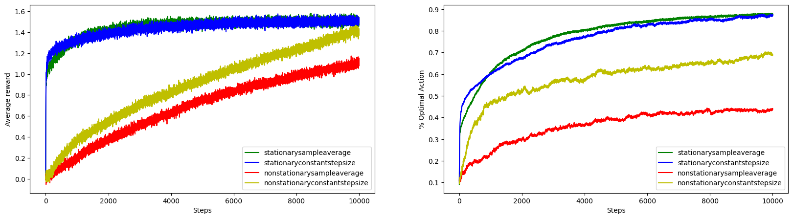
From the figure, we can see that both constant step size and sample average action value estimation methods shows comparable performance on stationary setting. However, in non-stationary setting, though lower than in stationary setting, the constant step size method performs significantly better than sample average method.
Optimistic Initial Values
Optimistic initial values is a technique used in the multi-armed bandit problem to encourage exploration in the early stages of learning. Instead of starting with initial action values set to zero or a neutral value, this approach sets the initial action values to a high, optimistic value, sometimes even higher than the maximum possible reward.
The optimistic initial values encourage exploration because the agent is initially biased to believe that all actions have high rewards. As the agent selects actions and receives actual rewards, it updates its estimates, and the optimistic values gradually fall towards their true values. This process continues until the value estimates of suboptimal actions fall below the estimates of the optimal action, and the agent starts exploiting the optimal action more frequently.
While optimistic initial values can be effective in stationary problems, there are some limitations to this approach. For instance, it is not well-suited for nonstationary problems, as its drive for exploration is temporary and may not adapt well to changes in the environment. Additionally, the technique relies heavily on the initial conditions, and finding the best initial values may require some trial-and-error or domain knowledge blog.
class OptimisticEpsilonGreedyAgent(EpsilonGreedyAgent):
    def __init__(self, k, runs, alpha=0.1, init_q=5, epsilon=0.1, random_state=None):
        """This behaves similar to epsilon greedy agent,
        but it starts with high optimistic action value."""
        super(OptimisticEpsilonGreedyAgent, self).__init__(k, runs, alpha, epsilon, random_state)
        self.init_q = init_q

        self.Q += self.init_q
Experiment 4: Optimistic Pure Greedy vs Epsilon Greedy
MultiArmedBanditTestBed.run_and_plot_experiments(
    steps=1000,  # To make spike clear
    exp_bandit_agent_dict={
        "optimisticgreedy": (
            StationaryMultiArmedBandit(k=k, runs=runs),
            OptimisticEpsilonGreedyAgent(k=k, runs=runs, alpha=0.1, init_q=5, epsilon=0)
        ),
        "realisticepsilongreedy": (
            StationaryMultiArmedBandit(k=k, runs=runs),
            EpsilonGreedyAgent(k=k, runs=runs, alpha=0.1, epsilon=0.01)
        ),
    },
)
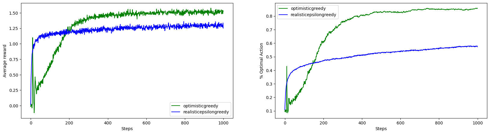
We can see that even with \(\epsilon=0\)(pure greedy) the agent with optimistic initial values outperforms \(\epsilon\)-greedy agent in the long run. Initially, it underperforms as it was forced to do exploration because of the optimistic values. Note that there is spike at about the 10th steps. The optimistic greedy policy promotes exploration in the initial steps, as all value estimates are set higher than their true values. This can lead to a scenario where the agent randomly selects the optimal action and then quickly abandons it in favor of other actions that have not been explored yet. This behavior results in a noticeable spike in performance around timestep 10, as the agent is still in the early stages of exploring different actions.
Experiment 5: Optimistic Pure Greedy vs Epsilon Greedy on Non-Stationary Setting
The experiment above for optimistic initial action values is done in stationary setting. Let’s run it in non-stationary setting see what happens.
MultiArmedBanditTestBed.run_and_plot_experiments(
    steps=10_000,
    exp_bandit_agent_dict={
        "optimisticgreedy": (
            NonStationaryMultiArmedBandit(k=k, runs=runs),
            OptimisticEpsilonGreedyAgent(k=k, runs=runs, alpha=0.1, init_q=5, epsilon=0)
        ),
        "realisticepsilongreedy": (
            NonStationaryMultiArmedBandit(k=k, runs=runs),
            EpsilonGreedyAgent(k=k, runs=runs, alpha=0.1, epsilon=0.01)
        ),
    },
)
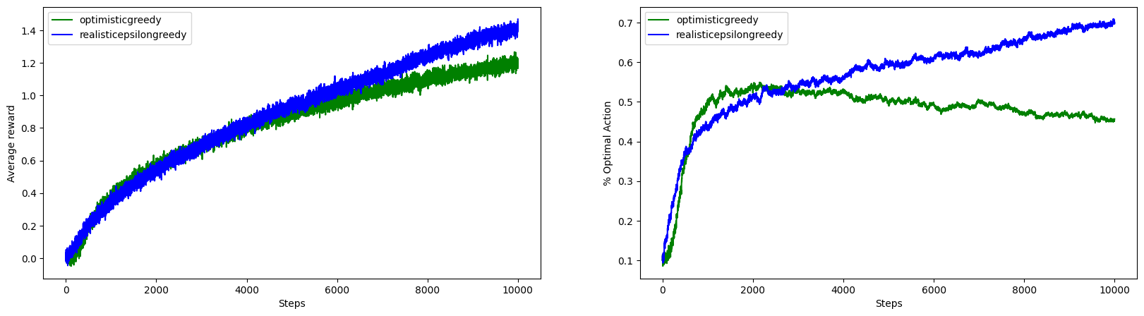
The experimenation clearly shows the limitation of the trick of using optimistic intial values to force exploration. It is not well suited to nonstationary problems because its drive for exploration is inherently temporary and non-stationary task at every steps creates need for exploration.
Experiment 6: Effects of Initial Action Values
Let’s run an experiment comparing different initial action value estimate.
MultiArmedBanditTestBed.run_and_plot_experiments(
    steps=5000,
    exp_bandit_agent_dict={
        "optimistic_egreedy_initq=500": (
            NonStationaryMultiArmedBandit(k=k, runs=runs),
            OptimisticEpsilonGreedyAgent(k=k, runs=runs, alpha=0.1, init_q=500, epsilon=0.01)
        ),
        "optimistic_egreedy_initq=5": (
            NonStationaryMultiArmedBandit(k=k, runs=runs),
            OptimisticEpsilonGreedyAgent(k=k, runs=runs, alpha=0.1, init_q=5, epsilon=0.01)
        ),
    },
)
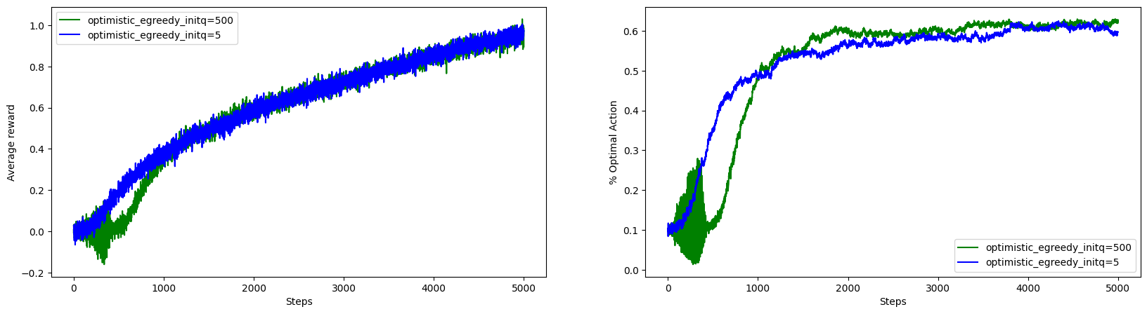
It is clear from the figure that the initial action value we choose has effects on beginning steps. With steps, the effect of initial values is lessened. I would like to quote the statements from the book here: “Indeed, any method that focuses on the initial conditions in any special way is unlikely to help with the general nonstationary case. The beginning of time occurs only once, and thus we should not focus on it too much.” So, for long one shouldn’t worry about the effect of initial action value choosen. But, there are tricks to avoid it and let’s explore one.
Unbiased Constant Step-Size
This trick given in the Exercise 2.7 of the Sutton’s book deals to avoid the effect of initial action values. The trick is to use step size: \(\beta \doteq \alpha /\overline{\omicron }_{n}\) where \(\overline{\omicron }_{n} \doteq \overline{\omicron }_{n-1} +\alpha ( 1-\overline{\omicron }_{n-1})\) for \(n \geq 0\), with \(\overline{\omicron}_{0}\doteq0\).
class UnbiasedEpsilonGreedyAgent(OptimisticEpsilonGreedyAgent):
    """Unbiased Constant Step-Size Agent.
    Inheritated from `OptimisticEpsilonGreedyAgent` to allow to set initial action values"""
    def __init__(self, k, runs, alpha=0.1, init_q=5, epsilon=0.1, random_state=None):
        super(UnbiasedEpsilonGreedyAgent, self).__init__(k, runs, alpha, init_q, epsilon, random_state)
        self.step_trace = np.zeros((self.runs, self.k))

    def get_step_size(self, action):
        """Calculate the step size for the given action using trace."""
        self.step_trace[np.arange(self.runs), action] += self.alpha*(1 - self.step_trace[np.arange(self.runs), action])
        return self.alpha / self.step_trace[np.arange(self.runs), action]
Experiment 7: Unbiased Constant Step-Size with Different Initial Action Values
Let’s run ubiased constant step-size agent with different inital values.
MultiArmedBanditTestBed.run_and_plot_experiments(
    steps=10000,
    exp_bandit_agent_dict={
        "unbiased_initq=500": (
            NonStationaryMultiArmedBandit(k=k, runs=runs),
            UnbiasedEpsilonGreedyAgent(k=k, runs=runs, alpha=0.1, init_q=500, epsilon=0.01)
        ),
        "unbiased_initq=5": (
            NonStationaryMultiArmedBandit(k=k, runs=runs),
            UnbiasedEpsilonGreedyAgent(k=k, runs=runs, alpha=0.1, init_q=5, epsilon=0.01)
        ),
    },
)
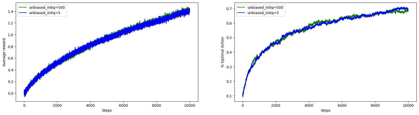
With this trick, we can see the effect of initial action values is gone. It is because with the unbiased constant step size the step size parameter for the first update will be \(1\) which means the agent will ignore the current action value estimate and set the estimate to the current reward it get.
Upper-Confidence Bound Action Selection
In above sections, we’re more focused in action value estimation methods. We explored sample average, constant step size and unbiased constant step size methods. Remember that a agent also has to make decision on what action to choose in each step. The greedy method always exploit the action with highest action value estimate it has till the current step, i.e., no exploration. The epsilon greedy method in each steps select the random action with some probability as way of doing exploration. While doing these random selection, equal preference is given not taking care of actions that are better than others.
Upper Confidence Bound (UCB) action selection methods aims to balance exploration and exploitation based on the confidence boundaries assigned to each action. The UCB algorithm is rooted in the principle of optimism in the face of uncertainty, meaning that the more uncertain we are about an action, the more important it becomes to explore that action. The UCB algorithm effectively solves the exploration-exploitation dilemma by selecting actions that maximize both the estimated reward and the exploration term. By doing so, it ensures that the agent explores uncertain actions while still exploiting actions with high estimated rewards, allowing it to learn the optimal action over time. Let’s implement it as it descibed in the section 2.7 of the book.
class UCBActionAgent(EpsilonGreedyAgent):
    def __init__(self, k, runs, alpha=0.1, confidence=1, random_state=None):
        self.k = k
        self.runs = runs
        self.alpha = alpha
        self.confidence = confidence
        self.random_state = random_state

        self.setup()

    def get_action(self):
        current_step = self.N.sum(axis=1, keepdims=True) + 1
        return np.argmax(
            self.Q + self.confidence * np.sqrt(
                np.log(current_step)/(self.N + 1e-5)  # To avoid divide by zero error
            ),
            axis=1
        )
Experiment 8: UCB vs \(\epsilon\)-Greedy on Stationary Setting
Let’s run an experiment comparing epsilon greedy with UCB with various confidence level.
MultiArmedBanditTestBed.run_and_plot_experiments(
    steps=1000,  # To make spike clear
    exp_bandit_agent_dict={
        "UCB C=1": (
            StationaryMultiArmedBandit(k=k, runs=runs),
            UCBActionAgent(k=k, runs=runs, alpha=0.1, confidence=1)
        ),
        "UCB C=2": (
            StationaryMultiArmedBandit(k=k, runs=runs),
            UCBActionAgent(k=k, runs=runs, alpha=0.1, confidence=2)
        ),
        "e-greedy, e=0.1": (
            StationaryMultiArmedBandit(k=k, runs=runs),
            EpsilonGreedyAgent(k=k, runs=runs, alpha=0.1, epsilon=0.1)
        ),
    },
)
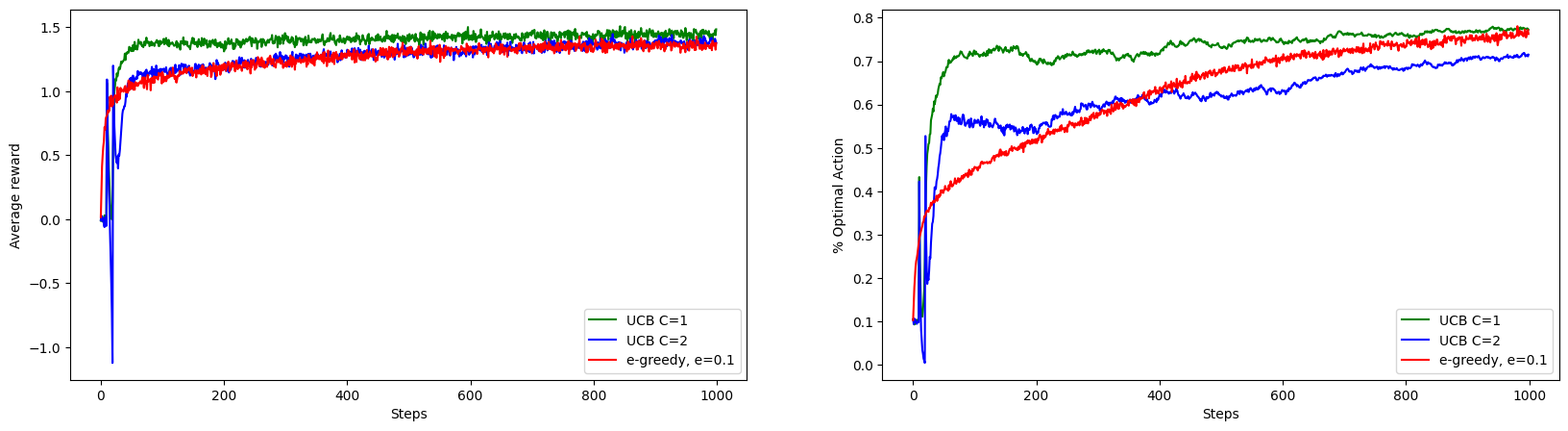
UCB with \(C=1\) is performing better than epsilon greedy but we didn’t see the imporovement with \(C=2\). This is because \(C\) controls the degree of exploration, higher the confidence level, higher the degree of exploration.
Experiment 9: UCB vs \(\epsilon\)-Greedy on Non-Stationary Setting
Let’s run the above experiment in non-stationary setting.
# e-greedy is better than UCB in nonstationary setting
MultiArmedBanditTestBed.run_and_plot_experiments(
    steps=10_000,
    exp_bandit_agent_dict={
        "UCB C=1": (
            NonStationaryMultiArmedBandit(k=k, runs=runs),
            UCBActionAgent(k=k, runs=runs, alpha=0.1, confidence=1)
        ),
        "e-greedy, e=0.1": (
            NonStationaryMultiArmedBandit(k=k, runs=runs),
            EpsilonGreedyAgent(k=k, runs=runs, alpha=0.1, epsilon=0.1)
        ),
    },
)
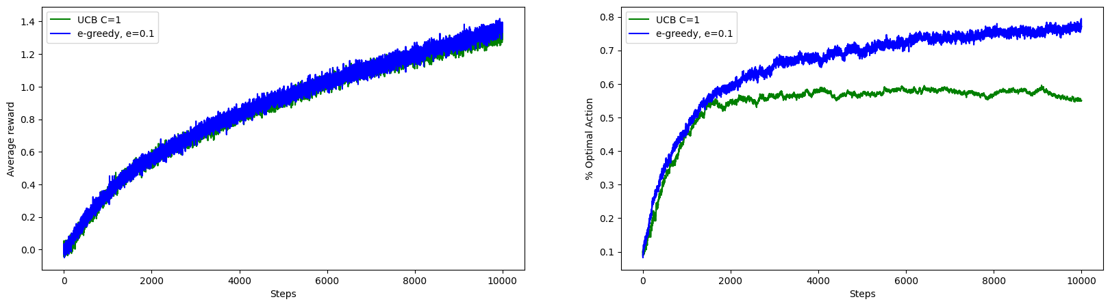
This experiments shows the limitation of UCB in non-stationary setting.
Gradient Bandit Algorithms
Instead of indiscriminately choosing actions or using some uncertainities values for exploring actions, a more sophisticated way is to learn the preference of each action. Agent can do so by using gradient bandit algorithms. Unlike other bandit algorithms that maintain an action-value estimate for each action, gradient bandit algorithms maintain a preference value for each action and use a soft-max distribution to derive the probabilities of selecting each action.
The core idea of gradient bandit algorithms is to update the preferences based on the received rewards and a baseline reward value, which can be the average of all observed rewards so far. The update rule is designed to increase the preference for actions that yield higher rewards than the baseline and decrease the preference for actions with lower rewards.
In each iteration, the agent selects an action according to the soft-max distribution derived from the action preferences and updates the preferences based on the received reward and the baseline. This process continues until the agent converges towards the optimal action or a stopping criterion is met. Gradient bandit algorithms can adapt to changing environments and provide a good balance between exploration and exploitation.
class GradientAgent(EpsilonGreedyAgent):
    """Gradient Bandit Algorithm"""
    def __init__(self, k, runs, alpha=0.1, random_state=None):
        self.k = k
        self.runs = runs
        self.alpha = alpha
        self.random_state = random_state

        self.setup()

    def setup(self):
        """Set up the initial preference and average reward for the GradientAgent"""
        self.nprandom = np.random.RandomState(self.random_state)
        # initial preference is same for all actions
        self.H = np.zeros((self.runs, self.k))
        self.avg_R = np.zeros((self.runs,))

    def action_proba(self):
        """Calculate the probability of each action."""
        exp = np.exp(self.H)
        prob = exp/exp.sum(axis=1, keepdims=True)

        # Persist for update method
        self.current_action_prob = prob
        return prob

    def get_action(self):
        """Get the action to take based on the action probabilities."""
        prob = self.action_proba()
        # TODO find better way to vectorize the following.
        return np.apply_along_axis(
            lambda row: self.nprandom.choice(np.arange(self.k), p=row),
            arr=prob,
            axis=1,
        )

    def update(self, action, reward):
        """Update the preferences and average reward based on the given action and reward."""
        step_size = self.get_step_size(action)

        # Get already calculated action probability if available
        prob  = self.current_action_prob if hasattr(self, "current_action_prob") else self.action_proba()
        prob = -prob
        prob[np.arange(self.runs), action] = 1 + prob[np.arange(self.runs), action]
        deltaR = reward - self.avg_R

        self.H += step_size*prob*deltaR[:, np.newaxis]
        self.avg_R += step_size*deltaR
Experiment 10: Gradient Bandit on Stationary Setting
MultiArmedBanditTestBed.run_and_plot_experiments(
    steps=1000,
    exp_bandit_agent_dict={
        "gradient": (
            StationaryMultiArmedBandit(k=k, runs=runs),
            GradientAgent(k=k, runs=runs, alpha=0.1)
        ),
        "e-greedy, e=0.01": (
            StationaryMultiArmedBandit(k=k, runs=runs),
            EpsilonGreedyAgent(k=k, runs=runs, alpha=0.1, epsilon=0.01)
        ),
    },
)
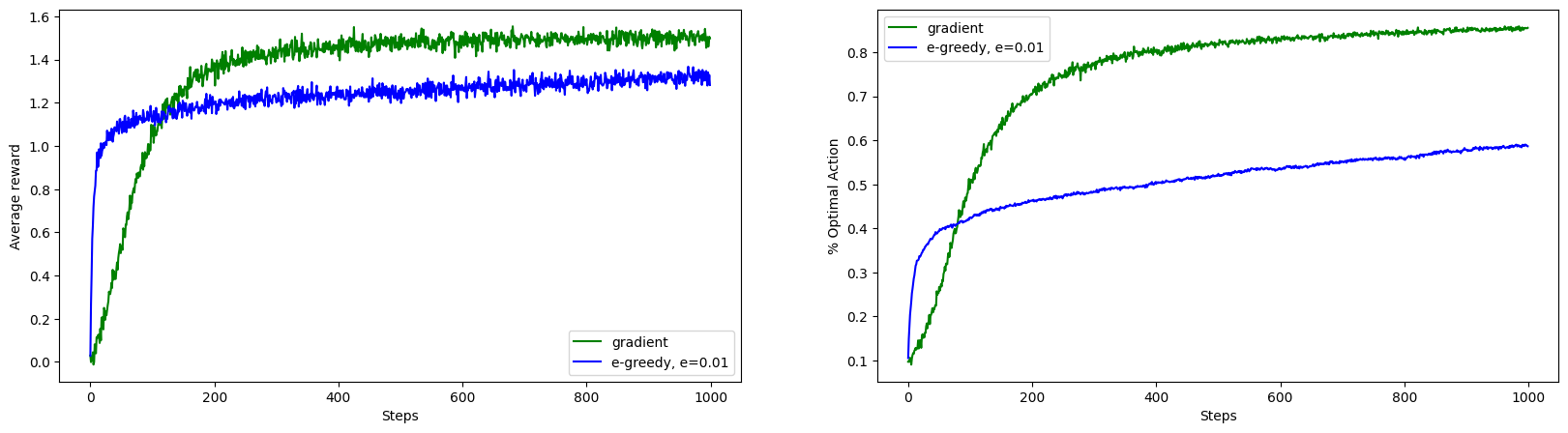
We can see almost 100% improvement in the optimal action selection because of gradient bandit algorithm.
Experiment 11: Gradient Bandit on Non-Stationary Setting
MultiArmedBanditTestBed.run_and_plot_experiments(
    steps=1000,
    exp_bandit_agent_dict={
        "gradient": (
            NonStationaryMultiArmedBandit(k=k, runs=runs),
            GradientAgent(k=k, runs=runs, alpha=0.1)
        ),
        "e-greedy, e=0.01": (
            NonStationaryMultiArmedBandit(k=k, runs=runs),
            EpsilonGreedyAgent(k=k, runs=runs, alpha=0.1, epsilon=0.01)
        ),
    },
)
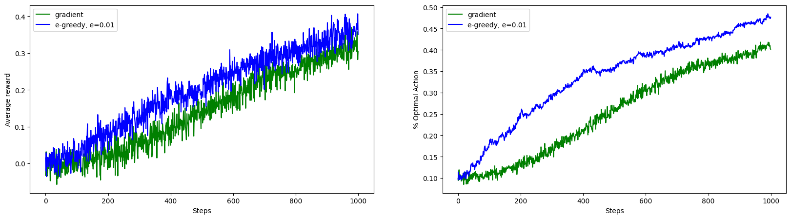
The gradient bandit algorithm also struggles in non-stationary setting.
This concludes the blog on multi-armed bandit problems. We implemented and compared various action value estimation and selection algorithms in sationary and non-stationary settings. All experiments showed the inherent challenge of exploitation vs exploration delimma in reinforcement learning.
References:
- Sutton, R. S., & Barto, A. G. (2018). Reinforcement Learning, second edition: An Introduction. MIT Press.